Fifth calibration
example - Calibrating a stereo system, stereo image rectification and 3D stereo triangulation
This example shows how to use the toolbox for calibrating a stereo system (intrinsically and extrinsically) and use the result of stereo calibration for stereo image rectification and 3D stereo triangulation.
Download the stereo data set stereo_example.zip (853Kb zipped) consisting of 14 pairs of corresponding left and right images.
The images are named left01.jpg,...,left14.jpg and right01.jpg,...,right14.jpg.
The package contains the two individual calibration results files Calib_Results_left.mat and Calib_Results_right.mat produced after separately calibrating the two cameras using the standard procedure described in the first example. The only difference is that after each calibration, the calibration result file Calib_Results.mat has been renamed to either Calib_Results_left.mat for the left camera or Calib_Results_right.mat for the right camera.
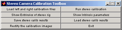
Run the main stereo calibration toolbox by typing stereo_gui in the main matlab window.
The toolbox window should turn into:
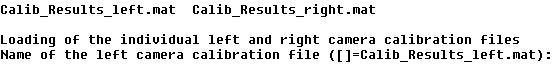
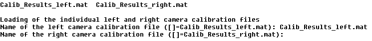
From within the folder containing the stereo data, click on the first button of the stereo toolbox Load left and right calibration files. The main matlab window will prompt you for the left and right camera calibration files:
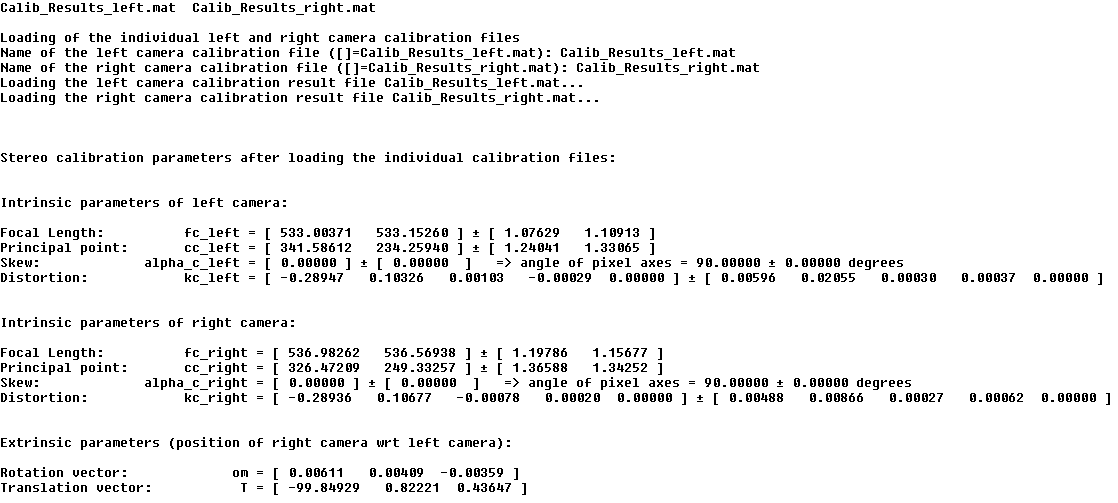
Enter Calib_Results_left.mat for the left camera calibration result file name:
Enter Calib_Results_right.mat for the right camera calibration result file name:
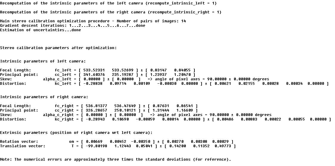
The initial values for the intrinsic camera parameters are shown in addition to an estimate for the extrinsic parameters om and T characterizing the relative location of the right camera with respect to the left camera. The intrinsic parameters fc_left, cc_left, alpha_c_left, kc_left, fc_right, cc_right, alpha_c_right and kc_right are equivalent to the traditional parameters fc, cc, alpha_c and kc defined on the parameter description page. The two pose parameters om and T are defined such that if we consider a point P in 3D space, its two coordinate vectors XL and XR in the left and right camera reference frames respectively are related to each other through the rigid motion transformation XR = R * XL + T, where R is the 3x3 rotation matrix corresponding to the rotation vector om. The relation between om and R is given by the rodrigues formula R = rodrigues(om).
Run the global stereo optimization procedure by clicking on the button Run stereo calibration in the stereo toolbox.
Observe that all intrinsic and extrinsic parameters have been recomputed, together with all the uncertainties so as to minimize the reprojection errors on both camera for all calibration grid locations. You may observe that the uncertainties on the intrinsic parameters (especially that of the focal values) for both cameras are smaller after stereo calibration. This is due to the fact that the global stereo optimization is performed over a minimal set of unknown parameters. In particular, only one pose unknown (6 DOF) is considered for the location of the calibration grid for each stereo pair. This insures global rigidity of the structure going from left view to right view. By default, the stereo optimization will recompute the intrinsic parameters for both left and right cameras. However, it may sometime be desirable to not re-optimize over the left and/or right camera intrinsic parameters and keep those previously estimated. In this case, the user may set recompute_intrinsic_left and/or recompute_intrinsic_right to zero prior to running stereo calibration. For more information type in your main matlab window help go_calib_stereo.
In order to save the stereo calibration results in the file Calib_Results_stereo.mat, click on Save stereo calib results in the stereo toolbox.
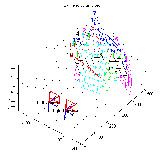
The spatial configuration of the two cameras and the calibration planes may be displayed in a form of a 3D plot by clicking on the button Show Extrinsics of the stereo rig in the stereo toolbox.
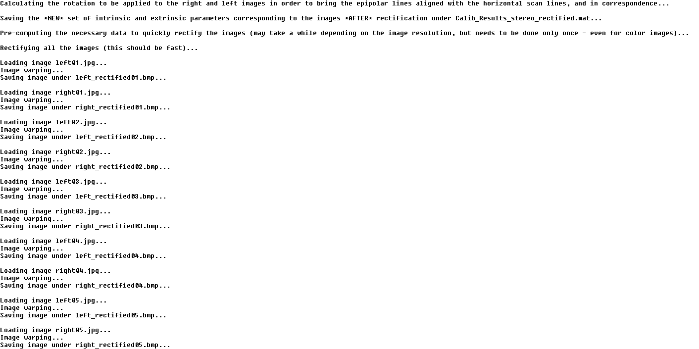
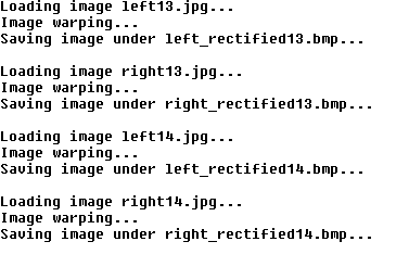
Finally, rectify the stereo images used for calibration by clicking on Rectify the calibration images. All 14 pairs of images are then stereo rectified (with epipolar lines matching with the horizontal scanned lines) under left_rectified01.bmp, right_rectified01.bmp,...,left_rectified14.bmp,right_rectified14.bmp.
In addition to generating the rectified images, the script also saves the new set of calibration parameters under Calib_Results_stereo_rectified.mat (valid only for the rectified images).
...
Since the original left and right images are provided, the two initial independent calibrations leading to the two result files Calib_Results_left.mat and Calib_Results_right.mat may also be done. Going through the corner extraction process, it is very important to keep in mind that for each pair, the same set of points must be selected in the left and right images. This means same grid of points and same origin point (to guarantee identical pattern reference frame). Therefore, it is crucial to make sure that the same origin point (first click) is consistently selected throughout. One simple technique is to always select the upper left corner of the grid as origin (this was done to generate the two provided calibration files). In your own stereo calibration, you may use a different strategy, such as marking the origin point on the grid pattern itself. For more information on the clicking rule for grid point selection, refer to the first calibration example.
Some additional information needed to complete the individual calibrations: the size of the squares in the grid is dX=dY=30mm and the window size parameters may be set to wintx=winty=7 for all images. After each calibration, remember to save the calibration results by clicking on Save and rename the file Calib_Results.mat to either Calib_Results_left.mat or Calib_Results_right.mat.
The toolbox also includes a function stereo_triangulation.m that computes the 3D location of a set of points given their left and right image projections. This process is known as stereo triangulation.
To learn about the syntax of the function type help stereo_triangulation in the main Matlab window.
As an exercise, let's apply the triangulation function on a simple example: let's re-compute the 3D location of the grids points extracted on the first image pair {left01.jpg, right01.jpg}. After running through the complete stereo calibration example, the image projections of the grid points on the right and left images are available in the variables x_left_1 and x_right_1. In order to triangulate those points in space, invoke stereo_triangulation.m by inputting x_left_1,x_right_1, the extrinsic stereo parameters om and T and the left and right camera intrinsic parameters:
The output variables Xc_1_left and Xc_1_right are the 3D coordinates of the points in the left and right camera reference frames respectively (observe that Xc_1_left and Xc_1_right are related to each other through the rigid motion equation Xc_1_right = R * Xc_1_left + T ). It may be interesting to see that one can then re-compute the "intrinsic" geometry of the calibration grid from the triangulated structure Xc_1_left by undoing the left camera location encoded by Rc_left_1 and Tc_left_1:
X_left_approx_1 = Rc_left_1' * (Xc_1_left - repmat(Tc_left_1,[1 size(Xc_1_left,2)]));
The output variable X_left_approx_1 is then an approximation of the original 3D structure of the calibration grid stored in X_left_1. How well do they match?